Integrating WaPOR and GEE for IGwA
| Site: | IHE DELFT OPENCOURSEWARE |
| Course: | On-the-Job Training for Palestine and Jordan |
| Book: | Integrating WaPOR and GEE for IGwA |
| Printed by: | Guest user |
| Date: | Friday, 22 May 2026, 6:16 AM |
Table of contents
- 1. Chapter 1:Introduction to Remote Sensing and Geospatial Tools for Agricultural Water Resource Analysis
- 2. Executive Summary
- 3. Chapter 2: Setting Up GEE Pipelines and Downloading WaPOR Data
- 4. Chapter 3: GEE and WaPOR: From Data Preprocessing to Analysis
- 5. Chapter 4: Modeling Irrigation Groundwater Dynamics: Abstraction and Recharge
- 6. Chapter 5: Model Validation -Spatial and Seasonal Analysis per field
- 7. Chapter 6: Model Calibration and Water Stress Indicators
- 8. Chapter 7: Introduction to IGwA dashboard
1. Chapter 1:Introduction to Remote Sensing and Geospatial Tools for Agricultural Water Resource Analysis
This chapter introduces foundational concepts critical for understanding and analyzing agricultural water resources using remote sensing technology, with a focus on the integration of advanced tools and methodologies (Section 1.1). It also offers an overview of the WaPOR v3 platform and Google Earth Engine (GEE), emphasizing their capabilities in assessing evapotranspiration, precipitation, and other water-related variables (Sections 1.2 and 1.3). Additionally, the chapter delves into the fundamentals of spatiotemporal analysis of groundwater dynamics in irrigated lands, including the analysis of groundwater abstraction for irrigation and recharge using well-established hydrological methods such as the Thornthwaite-Mather water balance method and FAO-based techniques (Section 1.4).
1.1. Role of Remote Sensing in Water Resource Management
1.2. Overview of WaPOR v3
- Overview of WaPOR and its applications in water resource management (OCW, Course: WaPOR introduction (version 3) | OCW IHE DELFT).
- Python for Geospatial Analyses using WaPOR Data (OCW, Topic: Introduction | Python for Geospatial Analyses using WaPOR Data | OCW IHE DELFT).
1.3. Overview of Google Earth Engine (GEE)
1.4. Fundamentals of IGwA
2. Executive Summary
The sustainable management of groundwater resources used in irrigated agricultural is increasingly critical in addressing global water scarcity and mitigating the impacts of climate change. This tutorial outlines the use of geospatial techniques and remote sensing data from FAO’s WaPOR and Google Earth Engine (GEE) tools, to estimate groundwater abstraction for irrigation and its recharge, assess water stress, and support decision-making for water resource management.
Key Highlights
Introduction to Remote Sensing and Analytical Tools
Remote sensing tools, such as WaPOR, and cloud-based platforms like GEE enable high-resolution spatial and temporal monitoring of water resources. These tools provide scalable and accessible methods for integrating diverse datasets into groundwater modeling and management, offering insights into hydrological processes.
Establishing GEE Pipelines and WaPOR Data Integration
The integration of WaPOR’s reference evapotranspiration and precipitation datasets with GEE’s soil property data forms a comprehensive pipeline. This enables efficient preprocessing, analysis, and visualization of hydrological data tailored to regional conditions. The pipeline facilitates seamless access and processing of data for subsequent modeling steps.
Data Preprocessing and Analysis with GEE and WaPOR
Advanced preprocessing techniques in GEE refine WaPOR datasets to create accurate and reliable inputs for groundwater modeling. The combined use of GEE and WaPOR streamlines data management, ensuring compatibility and usability for detailed water balance and recharge analyses.
Modeling Irrigation Groundwater Abstraction and Recharge
By using established methodologies like the Saxton & Rawls equations and Thornthwaite-Mather water balance calculations, soil hydraulic properties are derived. These parameters are critical for modeling infiltration, storage, and recharge processes across the vadose zone and aquifers, offering a clear understanding of groundwater dynamics in the irrigated agricultural sector.
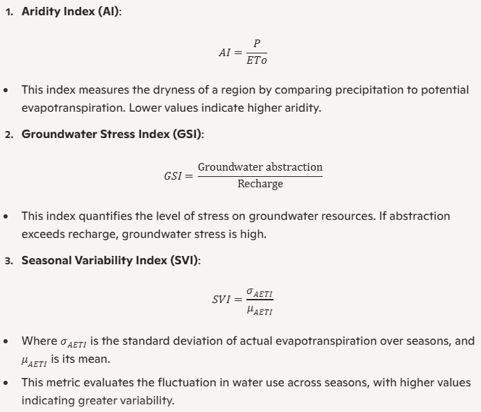
Model Validation, Calibration, and Stress Indicators
To improve model accuracy, advanced model calibration processes are needed to align crop-specific, soil-hydraulic, and irrigation system parameters with observed data. Validation ensures the integration of high-resolution spatial datasets accurately reflects real-world water fluxes. Additionally, water stress indicators, such as the Aridity Index (AI), Groundwater Stress Index (GSI), and Seasonal Variability Index (SVI), provide actionable insights into groundwater sustainability.
Spatial and Seasonal Analysis of Groundwater Dynamics
Calibrated models generate spatial distribution maps at the field-level and conduct seasonal analyses of groundwater use, enabling field-level decision-making. These insights are visualized through interactive dashboards, offering intuitive and dynamic representations of groundwater dynamics and aiding stakeholders in developing effective water management strategies.
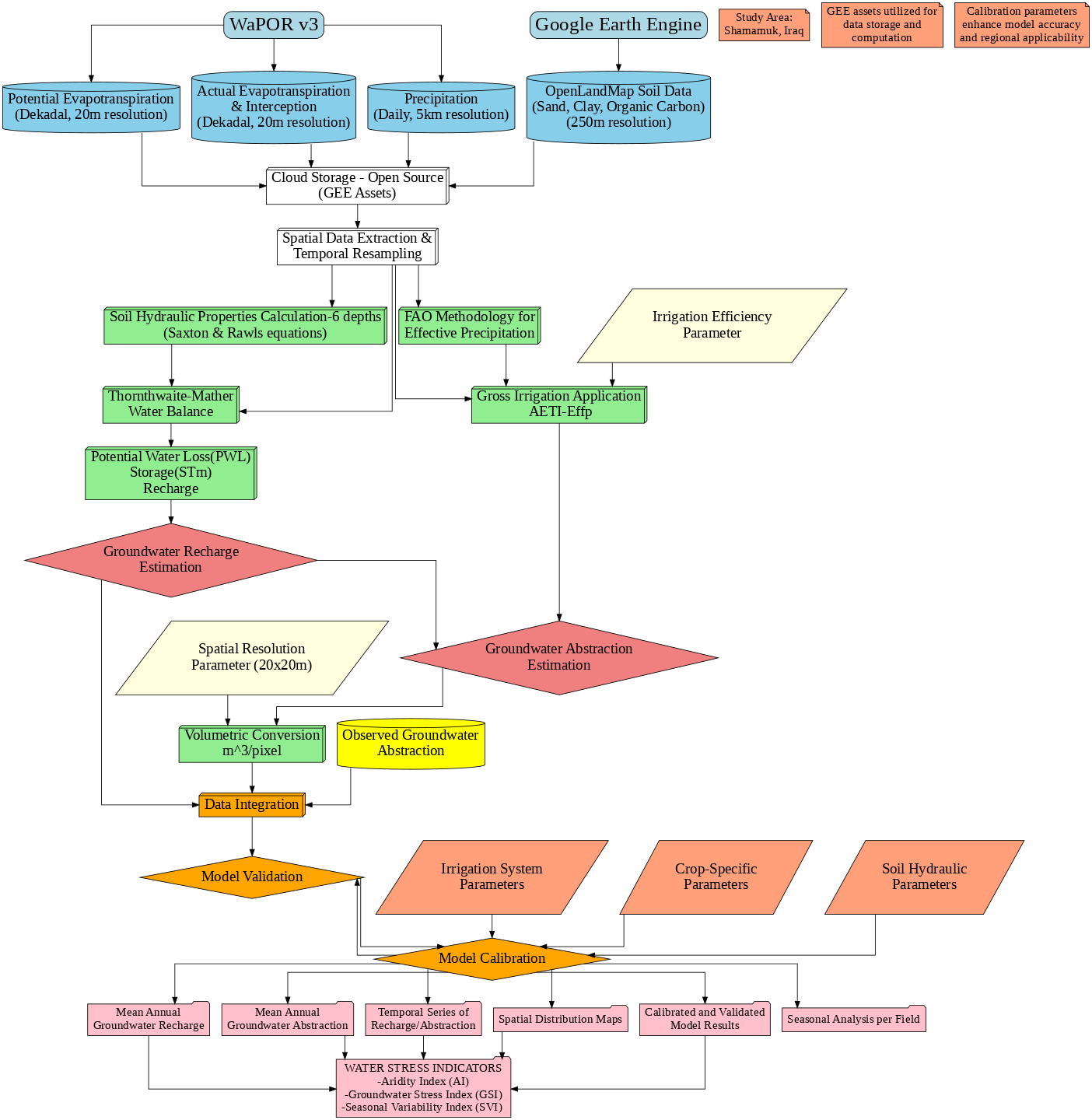
Model workflow Diagram
The methodology diagram showcases the integration of WaPOR, GEE, and observed data into a unified modeling framework. It highlights the systematic approach to groundwater abstraction for irrigation, recharge estimation, and model validation, culminating in decision-support outputs.
Conclusion
This tutorial provides a framework for leveraging remote sensing and computational tools to enhance groundwater resource management in the irrigated agricultural sector. By integrating high-resolution datasets, validated models, and actionable indicators, this approach offers scalable solutions to address the complexities of groundwater assessment in diverse regions. These methodologies could hold a significant potential for guiding sustainable practices in agricultural water use and addressing the challenges posed by water stress and climate change.
3. Chapter 2: Setting Up GEE Pipelines and Downloading WaPOR Data
This chapter provides a comprehensive guide to setting up Google Earth Engine (GEE) with a Google Cloud Project and integrating WaPOR L1 and 3 data processing pipelines. The primary goal is to establish a robust geospatial infrastructure that supports workflows for groundwater modelling assessment. By following the outlined steps, you will prepare the technical foundation for accessing, processing, and integrating high-resolution geospatial datasets from FAO's WaPOR platform into GEE.
The chapter is divided into three main sections:
-
Setting Up GEE with Google Cloud Project: This section details the prerequisites and step-by-step instructions for configuring your GEE environment, including account setup, API activation, and service account creation. It also covers initializing Earth Engine in Google Colab to facilitate programmatic data processing.
-
Adding Shapefiles as GeoJSON for Earth Engine: This section explains how to convert shapefiles into GeoJSON format and upload them to GEE as assets. This foundational step is crucial for defining areas of interest, clipping data, and supporting workflows such as groundwater analysis and dashboard development.
-
Accessing and Downloading WaPOR L3 Data: This section explores two methods for accessing and preparing WaPOR data—the manual approach using the wapordl package and the fully automated WaPOR v3 Geospatial Data Pipeline. Each method is described in detail, with a comparison to help you choose the best approach for your project.
Objectives
By the end of this chapter, you will:
-
Set up a functional GEE environment tailored to your project needs.
-
Configure authentication for accessing, clipping, and exporting multi-temporal WaPOR raster imagery.
-
Learn how to download and preprocess WaPOR L1 and 3 data using both manual and automated methods.
-
Convert shapefiles to GeoJSON and upload them as GEE assets for further geospatial analysis.
-
Gain insights into workflows that support efficient geospatial analysis for groundwater recharge and usage modeling.
Overview of the Process
The setup process addresses key technical challenges, including:
-
Accessing FAO WaPOR datasets for high-resolution geospatial analysis.
-
Managing multi-temporal raster imagery with consistent spatial resolutions and UTM zone-specific projections.
-
Preparing shapefiles as GeoJSON assets to enable advanced operations in GEE.
-
Automating or streamlining the extraction, preprocessing, and uploading of geospatial data to Earth Engine.
2.1 Setting Up GEE with Google Cloud Project
Prerequisites
- A Google Account
Step-by-Step Guide
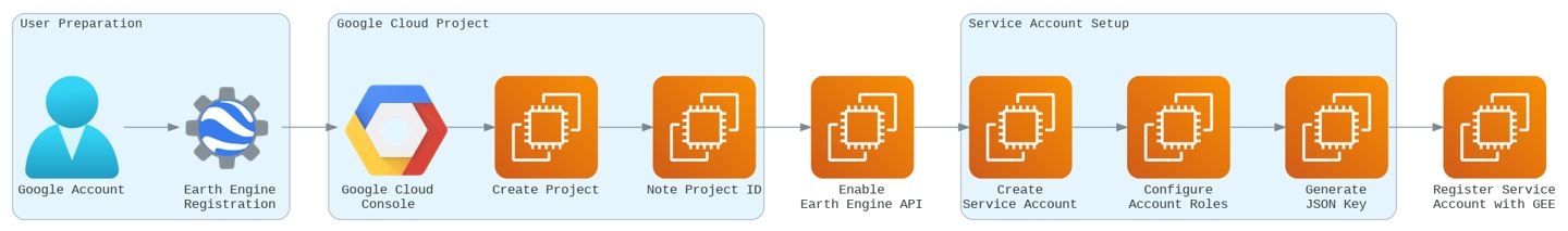
Step 1: Sign Up for Google Earth Engine ✍️
- Navigate to the Sign-Up Page: Go to the official Google Earth Engine website for noncommercial and research use: Google Earth Engine Sign-Up Page
- Select "noncommercial".
- Get Started: Click the "Get Started" button. You may be prompted to sign in with the Google account you wish to use.
** You will be redirected to the Google Cloud Console. Here, you'll link GEE to a Cloud project**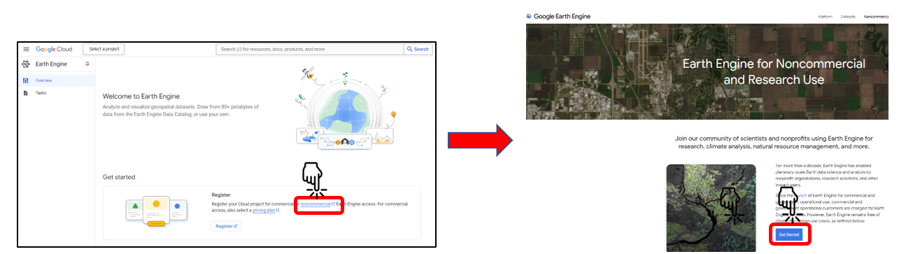
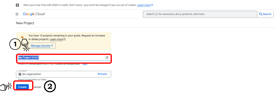
Step 2: Create and Select a Google Cloud Project ☁️
- Create a New Project: In the project selection dialog, click " New project"
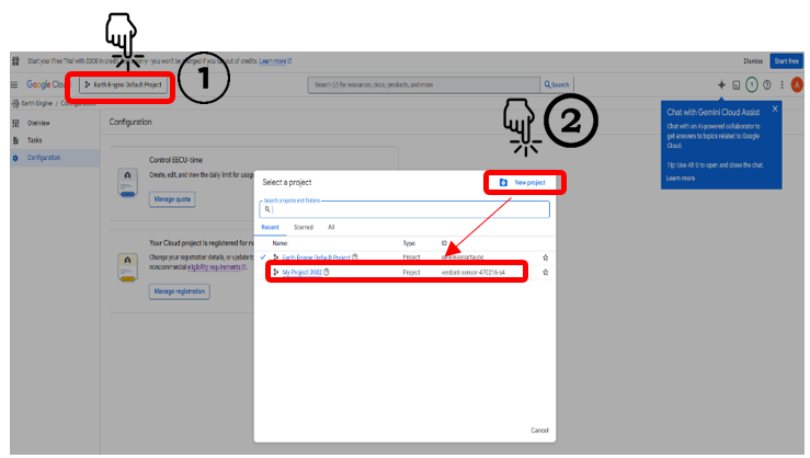
2. Enter Project Details:
-
-
Provide a unique
Project name (e.g.,
my-gee-project). -
If you're using a personal account, select
"No Organization".
-
Finalize Creation: Click "Create".
-
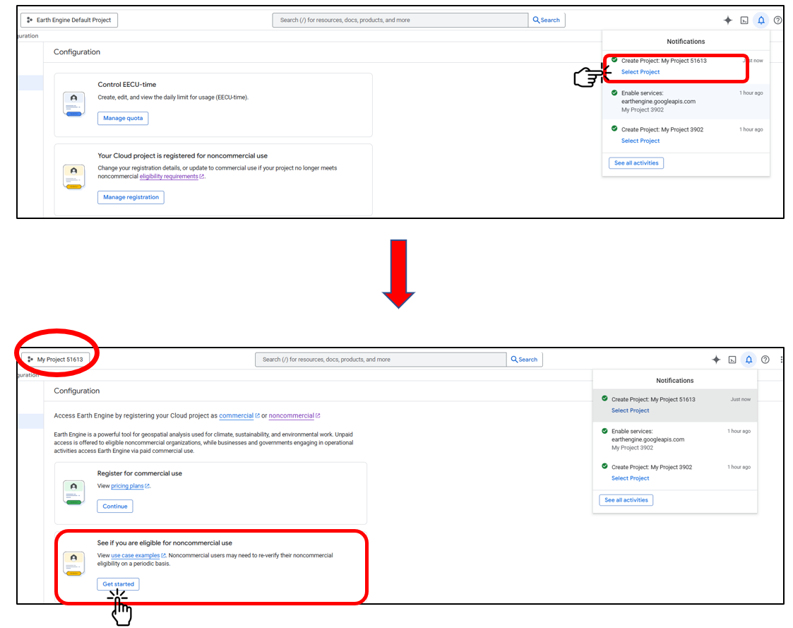
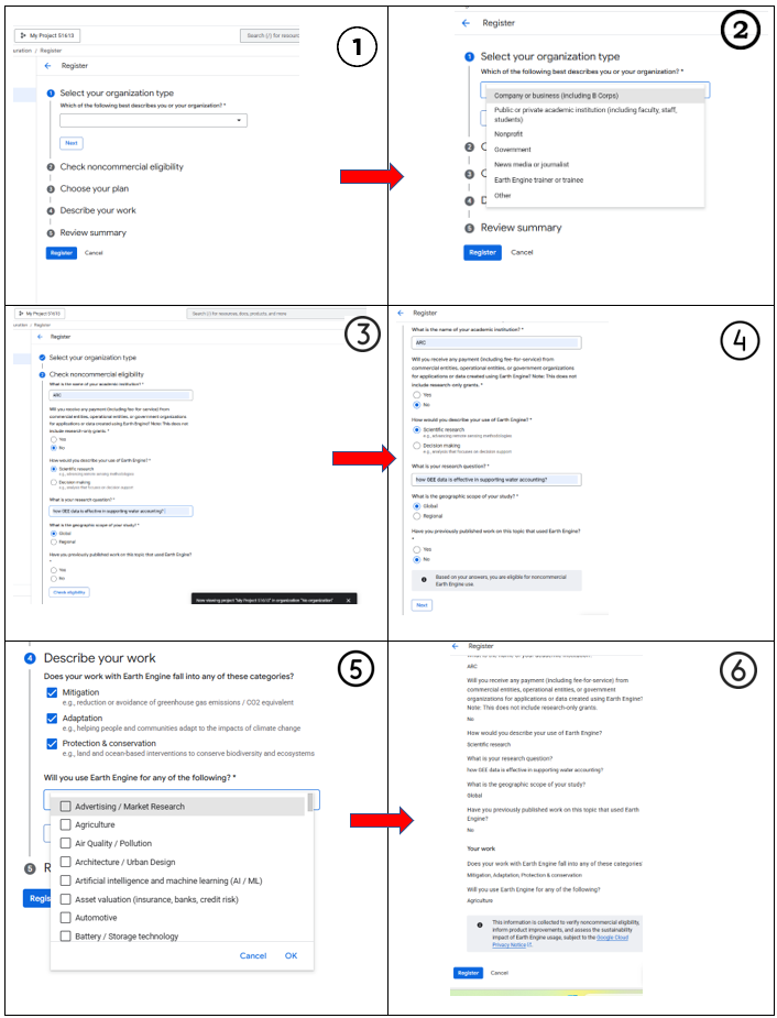
Step 3: Complete Noncommercial Registration Form 📝
1- Select Your Project
-
-
After clicking “Create” in the previous step, your project will appear in the Notifications menu.
-
Click on the project to open it.
-
Confirm that the project name is displayed in the Project Selection dialog at the top-right corner of the page.
-
2- Choose Your Plan
-
-
Review the eligibility criteria to ensure you qualify for the noncommercial plan.
-
Once confirmed, click “Get Started.”
-
3- Describe Your Work: Fill out the questionnaire detailing how you plan to use Earth Engine for your projects.
4- Review and Submit: Review the summary of your application and submit it.
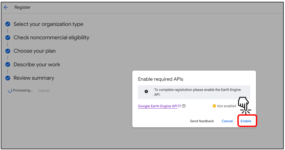
Step 4: Enable the Earth Engine API 🔌
To allow your project to communicate with GEE, you must enable the API.
-
Access the API: During the registration process, a dialog box will appear titled "Enable required APIs".
-
Enable the API: Ensure your new project is selected and click "Enable". Activation may take a few moments.
Step 5: Set Up the GEE Code Editor 🗂️
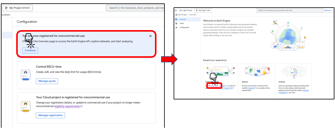
- Confirmation: Once enabled, you'll see a confirmation message that you are registered for noncommercial use. "Click Continue"
- Connect to Code Editor: Click on the "Code editor" icon (see second image), you will be redirected to the Earth Engine Code Editor page.
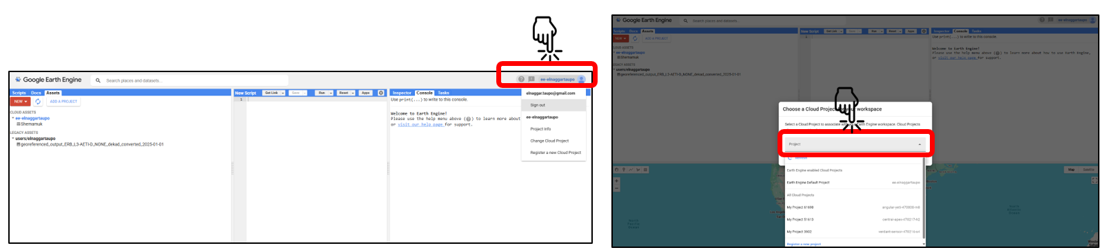
Step 6: Select a Cloud Project
-
Click the Project Selection Menu located in the top-right corner of the Earth Engine interface (highlighted in the first image).
-
From the dropdown menu, select “Change Cloud Project” or choose an existing project.
-
In the Choose a Cloud Project dialog (shown in the second image), click the Project dropdown and pick the project you want to associate with your Earth Engine workspace.
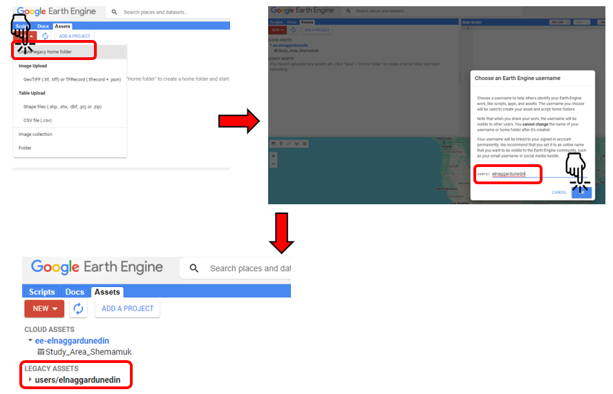
Step 7: Create a Legacy Asset
Legacy assets in Google Earth Engine serve as storage for processed images, which can later be utilized for tasks such as groundwater modeling.
-
Open the Assets Tab:
- Navigate to the Google Earth Engine interface and click on the Assets tab at the top of the page.
-
Initiate Legacy Asset Creation:
- Click the New button in the Assets tab.
- From the dropdown menu, select Create Legacy Home Folder to begin setting up your asset storage.
-
Set a Username for the Asset Folder:
- A dialog box will appear prompting you to choose an Earth Engine username.
- Enter your desired username (e.g., elnaggardunedin) and click OK.
-
Verify Legacy Asset Creation:
- Once created, the legacy asset folder will appear under the Legacy Assets section of the Assets tab (e.g.,
users/elnaggardunedin). - This folder will serve as a storage location for processed images generated during tasks like groundwater modeling.
- Once created, the legacy asset folder will appear under the Legacy Assets section of the Assets tab (e.g.,
Notes:
- The legacy asset folder is essential for managing and organizing outputs from your Earth Engine workflows, especially when dealing with large datasets or multiple processing steps.
- Ensure that the username you choose is appropriate and reflects your work, as it cannot be changed later.
- For effective storage management, consider organizing images into subfolders or collections based on project stages (e.g., preprocessing, modeling, and results).
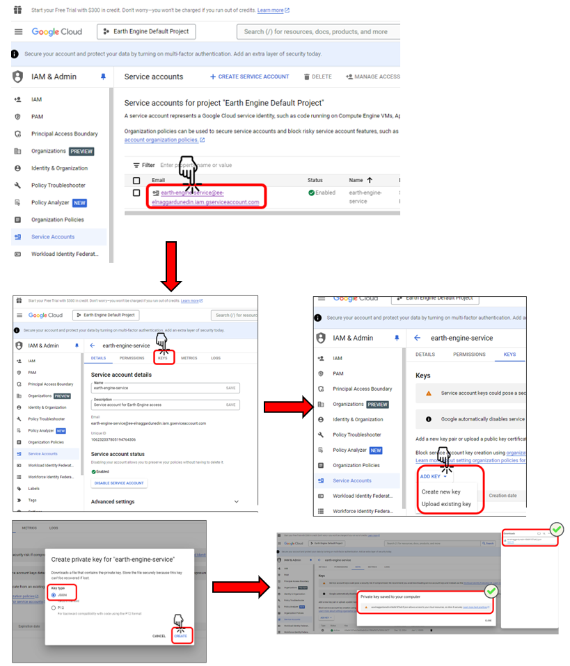
Step 8: Create and Configure a Service Account
- Open Service Accounts Section:
o In the Google Cloud Console, (https://console.cloud.google.com/) navigate to "IAM & Admin" > "Service Accounts."
- Create a New Service Account:
o Click "Create Service Account."
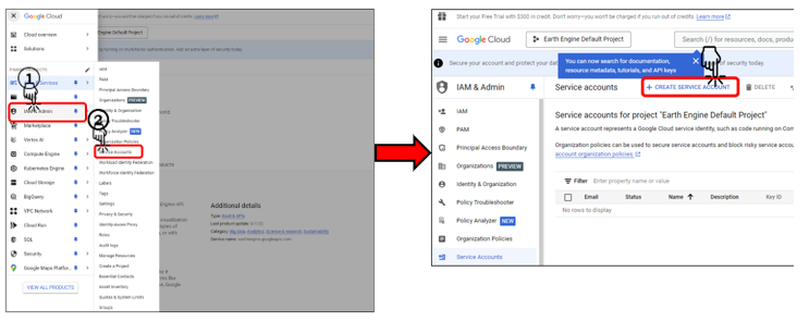
o Provide a name (e.g., "earth-engine-service") and description.
o Click "Create and Continue."
- Assign Required Roles:
o Add the following roles:
- "Owner"
- "Service Account User"
- "Earth Engine Resource Viewer"
o Click "Continue" and then "Done."

- Generate a JSON Key:
o Click on your new service account from the list.
o Go to the "Keys" tab and click "Add Key" > "Create New Key."
o Choose "JSON" format and download the key file on your local PC.
o Save the JSON file to a known and secure location on your local PC.
Step 9: Set Up Google Colab
-
Open a New Colab Notebook: Visit Google Colab and create a new notebook.

- Install Required Packages: Run the following commands in a code cell to install the necessary libraries:
!pip install earthengine-api
!pip install geemap
Step 10: Initialize Earth Engine in Colab
-
Import and Authenticate: Import the Earth Engine library and authenticate your Google account.
- Run the following code in a new cell:import ee # Authenticate Earth Engine access ee.Authenticate()- This will open a browser window prompting you to sign in and grant access permissions.
-
Initialize the Library:
Initialize Earth Engine with your project ID. Replaceyour-project-idwith the actual project ID. For example:# Replace with your project ID ee.Initialize(project='your-project-id') # Example: ee.Initialize(project='centering-sweep-439715-b3') # Verify the connection print('Earth Engine package initialized')````````````````````````````````````# Install required packages
!pip install earthengine-api
!pip install geemap````````````````````````````````# Import Earth Engine and authenticate
import ee
ee.Authenticate()``````````````````````````````````````````
# Initialize Earth Engine with your project ID
ee.Initialize(project='ee-enlaggardnudein)# Verify the connection
print('Earth Engine package initialized.')``````````````````````````````````````````````````````````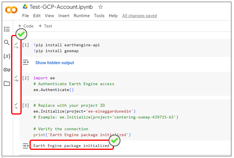
Step 11: Test Your Setup
- Run a Test Script:
Verify the setup by retrieving a satellite image and printing its metadata:# Retrieve a sample satellite image image = ee.Image('USGS/SRTMGL1_003') # Print image information print('Image information:', image.getInfo())``````````````````# Load a sample satellite image from Earth Engine
image = ee.Image("USGS/SRTMGL1_003")# Print metadata information about the image
print("Image information:", image.getInfo())``````````````````````````````````````````````````````````
If the setup is successful, you will see details of theUSGS/SRTMGL1_003image printed in the output.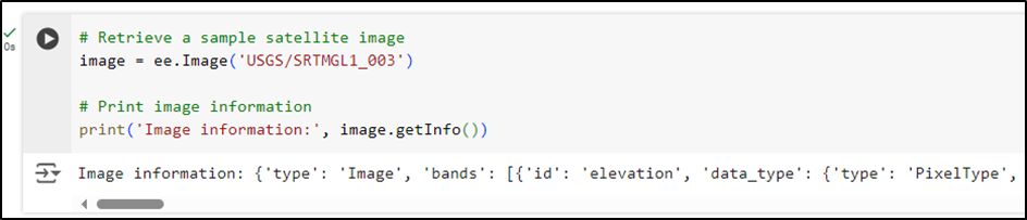
Troubleshooting Common Issues
1. Permission Denied (403) Error
If you encounter a 403 error, verify the following:
- Earth Engine API Activation: Ensure the Earth Engine API is enabled in your Google Cloud Project.
- Service Account Roles: Confirm that your service account has the required roles:
- Owner
- Service Account User
- Earth Engine Resource Viewer
- Service Account Registration: Check if the service account is registered with Earth Engine.
- Propagation Time: Allow 5–10 minutes after making changes for them to take effect.
2. Authentication Error
If authentication fails, try these steps:
- Correct Google Account: Ensure you are signed in with the correct Google account.
- Approval Confirmation: Verify that you have received the Earth Engine approval email.
- Service Account Verification: Check if the service account registration process is complete.
3. Project ID Error
If you experience a project ID error, follow these guidelines:
- Double-Check Project ID: Verify your project ID in the Google Cloud Console. Remember, the project ID is different from the project name.
- Copy Accuracy: Ensure you are copying the exact project ID.
- Allow Propagation: Wait a few minutes after creating the project before using it in Earth Engine.
Next Steps
Once your setup is successful, you can:
- Start utilizing Earth Engine data for your projects.
- Explore datasets in the Earth Engine Data Catalog.
- Learn from tutorials in the Google Earth Engine Documentation.
Important Reminder: Keep your authentication credentials secure and avoid sharing them publicly.
2.2 Adding Shapefiles as GeoJSON for Earth Engine
Purpose:
Shapefiles define areas of interest and are foundational for various geospatial tasks, such as downloading WaPOR data, clipping datasets, performing groundwater analysis, and creating development dashboards.
For best practice, shapefiles must first be converted to GeoJSON and uploaded as Earth Engine assets to be used in Google Earth Engine.
Reasons for Adding GeoJSON Assets to GEE :
-
Provides a central repository for AOI (Area of Interest) boundaries, enabling automated clipping of WaPOR data.
-
Supports integration into advanced workflows, such as groundwater modeling or dashboard development.
-
Simplifies spatial operations by leveraging GEE’s geospatial analysis capabilities.
By incorporating these steps into your workflow, you can efficiently manage spatial boundaries and automate geospatial processes for WaPOR datasets.

Python Script: Shapefile to JSON for Earth Engine Asset Upload
2.3 Accessing and Downloading WaPOR L1 and 3 Data
There are two primary methods for accessing and downloading WaPOR L3 data:
- Using the wapordl package to manually download WaPOR data, preprocess it, and upload it to GEE Assets.
- Leveraging the WaPOR v3 Automated Geospatial Data Pipeline, a Python-based solution that automates the entire workflow from data retrieval to GEE integration.
Below, we provide an explanation of both methods, including their features, workflows, and a comparison to help you determine the best approach for your project.
Method 1: wapordl Package
The wapordl package allows users to download WaPOR data directly to their local system or Google Cloud Drive. This method requires users to define the area of interest (via GeoJSON files or bounding box coordinates), specify the desired variables, and set the time period for the data. After downloading, users need to manually preprocess the data and upload it to GEE for further analysis.
Key Features of the wapordl Method:
- Flexible Downloading:
- Supports fetching WaPOR variables such as AETI, NPP, PCP, RET, and more.
- Allows defining areas of interest and selecting temporal resolutions (daily, dekadal, monthly, annual).
- Manual Preprocessing:
- Requires georeferencing and preparing data before uploading to GEE.
- Great for Small-Scale Projects:
- Ideal for users who want direct control over individual processing steps.
- Additional Steps for GEE Integration:
- Files must be uploaded to GEE assets manually after preprocessing.
Python Script: wapordl-Method
Method 2: WaPOR v3 Automated Geospatial Data Pipeline
The WaPOR v3 Automated Geospatial Data Pipeline streamlines the entire process of downloading, processing, and integrating WaPOR data into GEE assets. This Python script directly fetches data from FAO's WaPOR-Google Cloud Storage (L1 and 3 dataset), processes it with consistent projections, and uploads it to GEE assets without requiring any manual intervention.
Key Features of the Automated Pipeline:
- Automated Workflow:
- Fetches GeoTIFFs from FAO’s cloud storage and processes them into GEE assets automatically.
- Ensures consistency in projections (e.g., UTM zone) and georeferencing.
- Direct Integration with GEE:
- Eliminates the need to manually upload files to GEE, creating image collections automatically.
- Scalable and Efficient:
- Handles large datasets and long time series efficiently, processing data in daily, dekadal, monthly, and annual intervals.
- Error Handling:
- Includes retry mechanisms and monitoring to ensure smooth execution.
Python Script_level 3: WaPOR L3-AETI and E Raster Extraction, Clipping and Export via GEE
Python Script_Level 1: WaPOR L1-PCP Raster Data Extraction, Clipping and Export via GEE
4. Chapter 3: GEE and WaPOR: From Data Preprocessing to Analysis
This chapter builds upon the data collection methods introduced in the previous chapter (Chapter 2), shifting the focus to the preprocessing and analysis of spatiotemporal data that represent agricultural inputs and outputs to the atmosphere. These steps are essential for preparing data to serve as inputs for the irrigation groundwater assessment model - next chapter (Chapter 4).
Objective of This Chapter
The steps in this chapter:
- Prepare and visualize geospatial datasets that capture interactions between the land and atmosphere.
- Extract temporal trends of key hydrological components like precipitation (PCP), actual evapotranspiration (AETI), and potential evapotranspiration (PET).
- Transform data into forms suitable as inputs for the groundwater model introduced in the subsequent chapter.
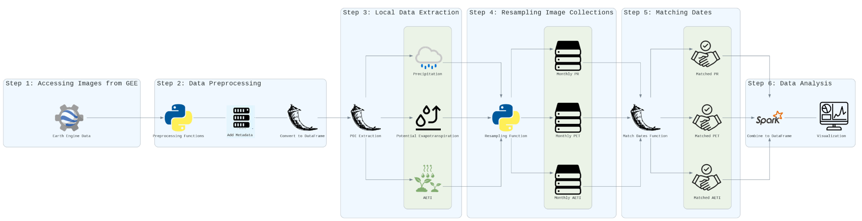
The workflow is organized into six key stages: accessing data, data preprocessing, local data extraction, resampling, date matching, and analysis. The following sections provide a detailed breakdown of each step, as illustrated in the diagram below.
Step-by-Step Guide
Step 1: Accessing Images from the Asset
- Objective: Retrieve WaPOR images for the study area, ensuring proper setup for further processing.
- Process:
- Use asset paths to load the required datasets (e.g., AETI, PET, and PCP) from WaPOR into the analysis environment.
- Verify dataset integrity by inspecting metadata and coverage to ensure compatibility with the study area.
- Perform any required reclassification or spatial adjustments to match the Point of Interest (POI).
Step 2: Data Preprocessing
- Objective: Transform raw datasets into structured, usable formats.
- Process:
- Apply preprocessing functions to clean and standardize the loaded datasets.
- Add metadata such as timestamps or geolocation to enrich the dataset for subsequent analysis.
- Convert the data into tabular DataFrame formats, making them compatible with downstream tools for aggregation and analysis.
Step 3: Local Data Extraction
- Objective: Extract relevant variables (e.g., AETI, PET, and PCP) for the study area or Point of Interest (POI).
- Process:
- Extract the following variables from the preprocessed datasets:
- Actual Evapotranspiration (AETI): Represents water loss to the atmosphere.
- Potential Evapotranspiration (PET): Indicates the maximum potential evaporation under ideal conditions.
- Precipitation (PCP): Reflects water input to the system.
- Ensure alignment of the extracted data spatially with the study area's boundaries to ensure accurate local analysis.
- Extract the following variables from the preprocessed datasets:
Step 4: Resampling Image Collections
- Objective: Standardize datasets by aggregating them over consistent time intervals (e.g., monthly or seasonal).
- Process:
- Use resampling functions to convert dekadal or irregular data into monthly aggregates.
- Generate resampled datasets for each key variable:
- Monthly AETI: Aggregated actual evapotranspiration.
- Monthly PET: Aggregated potential evapotranspiration.
- Monthly PCP: Aggregated precipitation.
- The resulting datasets are now temporally uniform and ready for further comparative analysis.
Step 5: Matching Dates
- Objective: Ensure all datasets are temporally aligned to enable consistent analysis and modeling.
- Process:
- Apply a date-matching function to synchronize datasets such as AETI, PET, and PCP.
- The output consists of matched datasets (e.g., Matched AETI, Matched PET, Matched PCP) with uniform timeframes.
Step 6: Data Analysis
- Objective: Combine processed datasets into a single structure for preliminary analysis and visualization.
- Process:
- Integrate the matched datasets into a consolidated DataFrame, ready for model input.
- Perform exploratory data analysis (EDA) to identify trends, seasonal patterns, or anomalies.
- Create visualizations to communicate key insights effectively.

Python Script: WaPOR_and_GEE_Data_Preprocessing_to_Analysis
5. Chapter 4: Modeling Irrigation Groundwater Dynamics: Abstraction and Recharge
This chapter focuses on understanding groundwater use for irrigation and recharge processes in agricultural areas, offering insights into their dynamics, quantification methodologies, and practical applications for sustainable water resource management in this critical sector.
Groundwater abstraction for irrigation constitutes one of the largest consumptive uses of this resource, driven by the need to meet crop water requirements. Accurately estimating abstraction volumes involves analyzing irrigation practices, crop water needs, and local precipitation patterns. Equally important is groundwater recharge—the process of replenishing aquifers through infiltration and percolation—which ensures the long-term sustainability of these systems. Recharge in agricultural settings is influenced by soil properties, irrigation return flows, precipitation, and evapotranspiration, all of which are dynamically shaped by natural variability and human interventions.
This chapter introduces a framework for estimating groundwater use and recharge in irrigated areas, leveraging preprocessed satellite-derived WaPOR v3 data (Chapter 3), soil hydraulic models, and the Thornthwaite-Mather water balance procedure. It also addresses key challenges, including accounting for spatial and temporal variability, improving irrigation efficiency, and assessing the impacts of climate change on groundwater dynamics. By integrating methodologies and future directions, the chapter aims to advance understanding of groundwater processes within the irrigated agricultural context, supporting efforts toward sustainable water management.
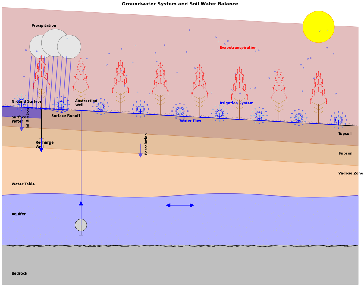
4.1. Groundwater System for Irrigation
The figure provides a foundational visualization of the hydrological processes involved in understanding groundwater systems and soil water balance, which directly supports the methodologies discussed in Sections 4.2 and 4.3. Groundwater abstraction for irrigation use, as highlighted in Section 4.2, is depicted in the diagram through the abstraction well, showing the extraction of water from the aquifer. To accurately calculate groundwater abstraction for irrigation, the model incorporates crop water requirements, irrigation efficiency, and precipitation—processes represented visually by the precipitation and the irrigation system in the topsoil layer. Additionally, evapotranspiration is a critical parameter influencing water demand, shown in the diagram through upward red arrows representing water loss from soil and plants. This interplay informs the need for effective classification methods like AETI, which refine crop-specific water estimates.
Similarly, Section 4.3's focus on Groundwater Recharge aligns with the recharge well and the downward movement of water from infiltration and percolation depicted in the vadose zone of the diagram. The processes of precipitation, infiltration, and soil moisture dynamics, visualized in the figure, are key inputs for the Thornthwaite-Mather water balance model. The calculation of soil hydraulic properties (e.g., wilting point and field capacity) is essential for estimating recharge rates and is conceptually tied to the soil stratification (topsoil, subsoil, and vadose zone) and water movement into the aquifer. This integrated perspective of recharge and abstraction ensures the sustainable management of groundwater resources, as described in the methodologies.
4.2. Methodology of IGwA
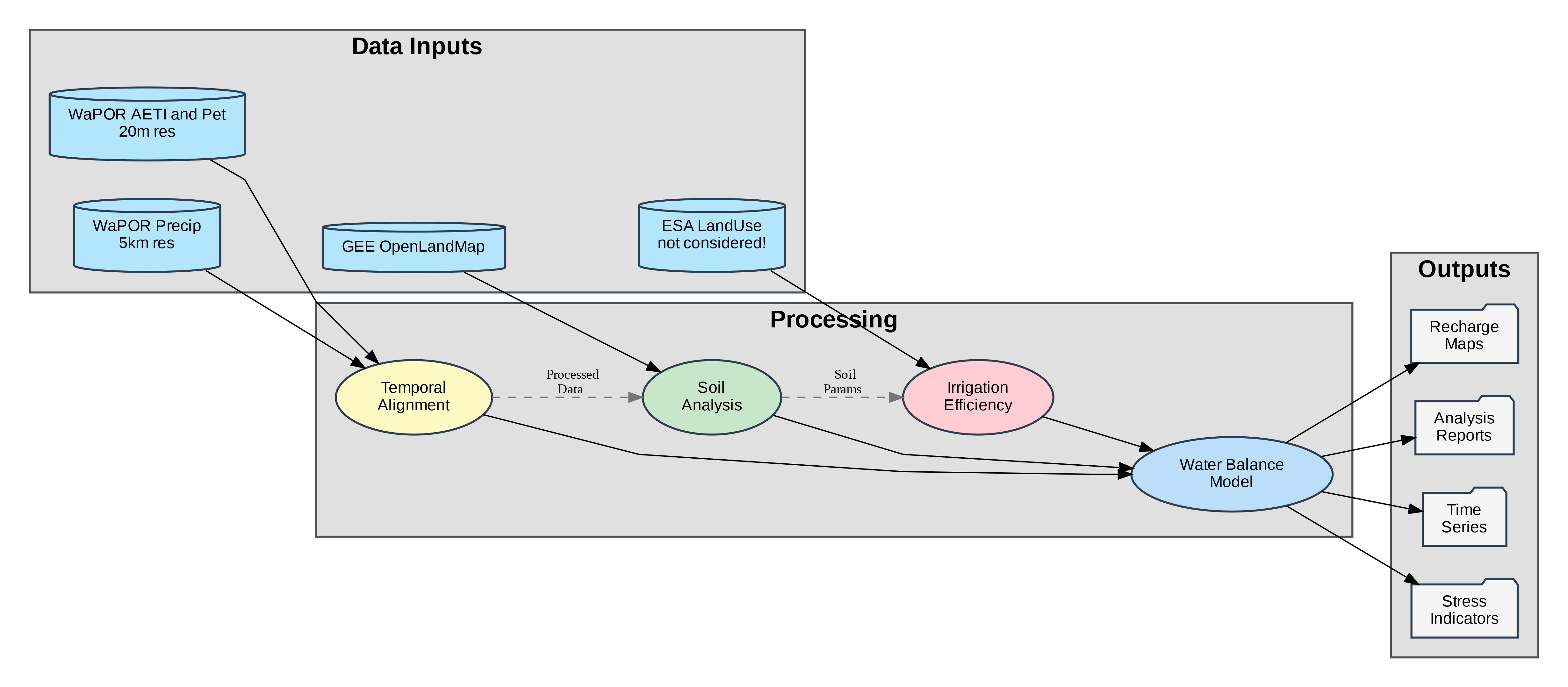
The following methodology provides a comprehensive framework for assessing groundwater dynamics in agricultural regions using remote sensing and hydrological modeling. The process begins with the integration of multi-source data, including high-resolution actual evapotranspiration (AETI) from WaPOR, daily precipitation from WaPOR, soil properties from GEE-OpenLandMap, and land-use classification from ESA (not included yet). These datasets are temporally aligned and spatially resampled to ensure consistency, forming the foundation for calculating critical parameters such as soil field capacity, wilting point, and irrigation efficiency. Key steps include the application of the Saxton & Rawls equations for soil hydraulic properties and crop-type-specific irrigation efficiency adjustments based on satellite-derived land-use data.
The core of the methodology employs an enhanced Thornthwaite-Mather water balance model to estimate groundwater recharge and abstraction. By analyzing the relationship between effective precipitation, potential evapotranspiration (PET), and soil moisture storage, the model iteratively calculates water deficits/surpluses while incorporating irrigation demands derived from AETI data. Irrigation efficiency is dynamically adjusted using crop-specific coefficients, improving the accuracy of abstraction estimates in arid agricultural systems.
The final outputs—including spatially explicit recharge maps, abstraction rate time series, and water stress indices—provide actionable insights for sustainable groundwater management. This approach enables policymakers to identify over-exploited zones, optimize irrigation schedules, and assess climate change impacts on water resources. By leveraging Google Earth Engine’s cloud-computing capabilities, the methodology balances high spatial resolution (20m) with computational efficiency, making it particularly suitable for large-scale agricultural water management in data-scarce regions. The integration of calibration parameters and uncertainty analysis ensures robustness, while user-friendly visualizations facilitate stakeholder engagement and evidence-based decision-making.
4.3. Groundwater Abstraction for Irrigation
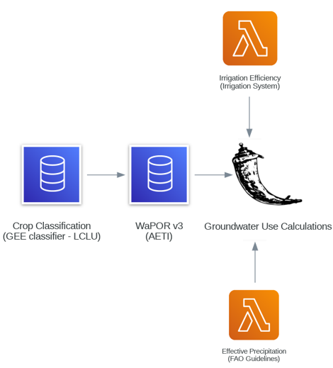
To estimate groundwater abstraction for irrigation purposes by analyzing crop water requirements, irrigation efficiency, and precipitation.
Methodology
The abstraction volume is calculated using crop water requirements, effective precipitation, and irrigation efficiency. Crop classification has to be the first step in determining water demand where a classification model is trained to identify crop types, with each type associated with specific water requirements. This process utilizes spectral-temporal statistics of satellite imagery. The classified crop map assigns water requirements.
In this model, the classification is considered by actual evapotranspiration (AETI) so the classifier procedures aren't implemented. While the model only incorporates AETI derived from WaPOR datasets, a significant area of improvement would be needed to involve dynamically linking AETI values to specific crop classifications. This could enhance the accuracy of water demand estimates and further refine the model.
4.4. Groundwater Recharge
To estimate groundwater recharge rates, incorporating precipitation, evapotranspiration, and soil moisture dynamics.
Methodology
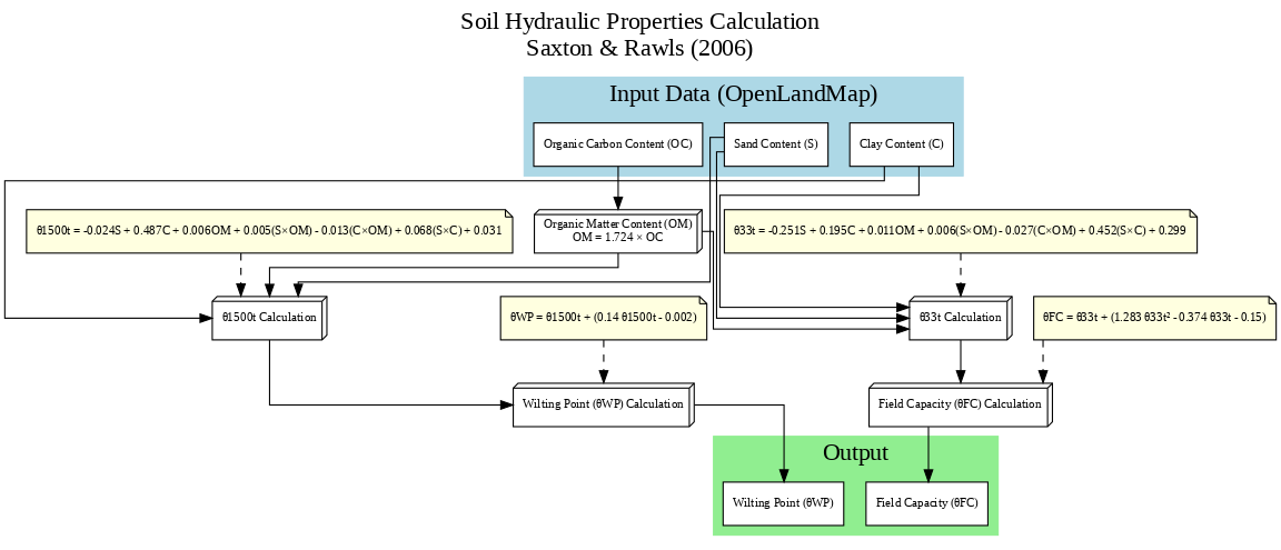
The following methodology integrates data from multiple sources and computational steps to estimate groundwater recharge using the Thornthwaite-Mather (TM) procedure. It begins with soil profile data obtained from OpenLandMap through Google Earth Engine (GEE) collections. This data undergoes preprocessing to adapt it for further analysis. Then, soil hydraulic properties such as wilting point and field capacity are calculated using the Saxton & Rawls (2006) approach. The results are utilized to determine the soil's hydraulic properties. Simultaneously, water availability data, including precipitation and potential evapotranspiration (PET), is derived from WaPOR v3. The computed soil and water data are combined in the TM procedure to model groundwater recharge.
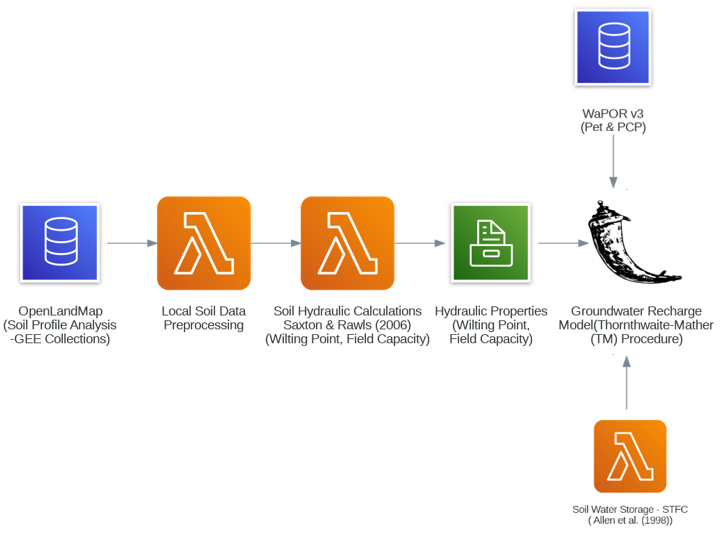
4.4.1 Hydraulic Properties (FC&WP) via Saxton-Rawls Model
OpenLandMap datasets are used to describe clay, sand and organic carbon content of soil. A global dataset of soil water content at the field capacity with a resolution of 250 m has been made available by Hengl & Gupta (2019). However, up to now, there is no dataset dedicated to the water content of soil at the wilting point. Consequently, in the following, both parameters will be determined considering the previous equations and using the global datasets giving the sand, clay and organic matter contents of the soil. According to the description, these datasets are based on machine learning predictions from global compilation of soil profiles and samples. Processing steps are described in detail here. The information (clay, sand content, etc.) is given at 6 standard depths (0, 10, 30, 60, 100 and 200 cm) at 250 m resolution.
Two key hydraulic properties of soil are utilized:
- the wilting point refers to the moisture level below which plants are unable to extract water through their roots.
- the field capacity marks the maximum moisture level that soil can retain. Beyond this point, gravitational forces prevail, causing water to percolate into deeper soil layers.
Equations developed by Saxton & Rawls (2006) are applied to correlate these parameters with soil texture. The wilting point water content, denoted as θWP, is calculated using the following formula:
with:
where:
- S: indicates the percentage of sand in the soil (by mass),
- C: represents the percentage of clay in the soil (by mass),
- OM: refers to the percentage of organic matter in the soil (by mass).
Likewise, the water content at field capacity, symbolized as θFC, is computed using this equation:
with:
Now that soil properties are described, the water content at the field capacity and at the wilting point can be calculated according to the equation defined at the beginning of this section. Please note that in the equation of Saxton & Rawls (2006), the wilting point and field capacity are calculated using the Organic Matter content (OM) and not the Organic Carbon content (OC). In the following, we convert OC into OM using the corrective factor known as the Van Bemmelen factor:
0M=1.724×OC
4.4.2 Soil Water Storage (STFC)
The soil water storage is calculated as outlined by Allen et al. (1998) (the document can be downloaded here):
TAW=1000×(θFC−θWP)×Zr
where:
- TAW: the total available soil water in the root zone [mm],
- θFC: the water content at the field capacity [m3m−3],
- θWP: the water content at wilting point [m3m−3],
- Zr: the rooting depth [m],
Typical values of θFC and θWP for different soil types are given in Table 19 of Allen et al. (1998).
The readily available water (RAW) is given by RAW=p×TAW, where p is the average fraction of TAW that can be depleted from the root zone before moisture stress (ranging between 0 to 1). This quantity is also noted as soil water storage (STFC) which is the available water stored at field capacity in the root zone.
Ranges of maximum effective rooting depth Zr, and soil water depletion fraction for no stress p, for common crops are given in the Table 22 of Allen et al. (1998). In addition, a global effective plant rooting depth dataset is provided by Yang et al. (2016) with a resolution of 0.5° by 0.5° (see the paper here and the dataset here).
According to this global dataset, the effective rooting depth around our region of interest can reasonably assumed to Zr=0.5. Additionally, the parameter p is also assumed constant and equal to and p=0.5 which is in line with common values described in Table 22 of Allen et al. (1998).
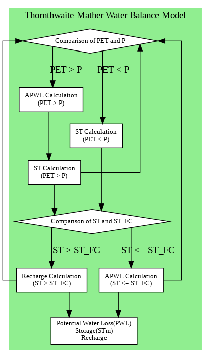
4.4.3 Thornthwaite-Mather (TM) Water Balance Model
The Thornthwaite-Mather procedure used to estimate groundwater recharge is explicitly described by Steenhuis and Van der Molen (1985). This procedure uses monthly sums of potential evaporation, cumulative precipitation, and the moisture status of the soil which is calculated iteratively. The moisture status of the soils depends on the accumulated potential water loss (PWL). This parameter is calculated depending on whether the potential evaporation is greater than or less than the cumulative precipitation. The procedure reads as follow:
The workflow follows these steps:
1. Comparison of PET and P:
- The first step compares Potential Evapotranspiration (PET) and Precipitation (P) to determine whether the demand for water (PET) exceeds the supply (P) or not:
-
Case 1: PET > P
- Water demand exceeds rainfall, triggering a calculation of APWL (Accumulated Potential Water Loss). This value tracks the cumulative water deficit due to evapotranspiration exceeding precipitation.
- Soil water storage (ST) is updated based on the deficit.
-
Case 2: PET < P
- Water supply exceeds demand, allowing for soil water storage (ST) replenishment.
-
2. Comparison of Soil Water Storage (ST) with Field Capacity (ST_FC):
- After calculating or updating ST, it is compared with the Field Capacity (ST_FC):
- Case 1: ST > ST_FC
- When soil water storage exceeds field capacity, excess water is considered as Recharge, contributing to groundwater.
- Case 2: ST ≤ ST_FC
- When soil water storage is below or equal to field capacity, APWL is updated.
- Case 1: ST > ST_FC
3. Outputs:
- Based on the above conditions, the model computes:
- Potential Water Loss (PWL): The water lost due to evapotranspiration when PET > P.
- Soil Storage (STm): The updated soil water storage level.
- Recharge: The water that contributes to replenishing groundwater when ST > ST_FC.
Use the following script to run the groundwater modeling using WaPOR and GEE

                                                      Python Script: Modeling Groundwater Abstraction for Irrigation and Recharge Using WaPOR and GEE

Python Script_ Palestine
Modeling IGwA Using WaPOR and GEE_Palestine
6. Chapter 5: Model Validation -Spatial and Seasonal Analysis per field
Subtitles:
5.1 Data Integration Techniques
5.2 Model Validation for Groundwater Analysis
5.3 Ensuring Data Reliability
Content:
- Integration of spatial and observational data for consistent modeling.
- Techniques to validate groundwater recharge and abstraction models.
- Methods for improving model reliability and accuracy.
Challenges and Future Directions
While this model provides a robust framework for estimating irrigation groundwater abstraction and recharge, certain limitations warrant further exploration:
-
Integration of AETI and Crop Classification: A direct link between AETI values and classified crop types can improve abstraction estimates.
-
Spatial and Temporal Variability: High-resolution data on irrigation practices and crop phenology can enhance temporal accuracy.
-
Irrigation Efficiency: Incorporating region-specific irrigation practices and efficiencies could refine the model further.
-
Soil Parameter Variability: Using global datasets introduces uncertainties due to regional variations in soil properties. More localized soil data could improve model accuracy.
-
Temporal Resolution: The iterative nature of the Thornthwaite-Mather procedure relies on monthly data, which may not capture finer temporal recharge dynamics. Higher-resolution temporal data would enhance precision.
-
Climate Variability: Recharge patterns are sensitive to changing precipitation and evapotranspiration trends under climate change scenarios. Adapting the model to account for these shifts is essential for future studies.
-
Interplay Between Abstraction and Recharge: High abstraction rates can reduce the soil moisture available for recharge. Coupling abstraction and recharge models more tightly could yield a more holistic understanding of groundwater dynamics.
7. Chapter 6: Model Calibration and Water Stress Indicators
Subtitles:
6.1 Calibration of Soil, Crop, and Irrigation System Parameters
6.2 Groundwater and Recharge Temporal Analysis
6.3 Water Stress Indicators
Content:
- Model calibration to refine parameters like soil hydraulics, irrigation systems, and crop-specific factors.
- Seasonal and temporal trends in recharge and abstraction.
- Overview of water stress indicators (AI, GSI, SVI).
8. Chapter 7: Introduction to IGwA dashboard
Jafr-Shoubak_Irrigation Groundwater Analysis Dashboard
Access the service via: Groundwater Analysis Dashboard_Jafr-Shoubak