Integrating WaPOR and GEE for IGwA

This chapter focuses on understanding groundwater use for irrigation and recharge processes in agricultural areas, offering insights into their dynamics, quantification methodologies, and practical applications for sustainable water resource management in this critical sector.

Groundwater abstraction for irrigation constitutes one of the largest consumptive uses of this resource, driven by the need to meet crop water requirements. Accurately estimating abstraction volumes involves analyzing irrigation practices, crop water needs, and local precipitation patterns. Equally important is groundwater recharge—the process of replenishing aquifers through infiltration and percolation—which ensures the long-term sustainability of these systems. Recharge in agricultural settings is influenced by soil properties, irrigation return flows, precipitation, and evapotranspiration, all of which are dynamically shaped by natural variability and human interventions.

This chapter introduces a framework for estimating groundwater use and recharge in irrigated areas, leveraging preprocessed satellite-derived WaPOR v3 data (Chapter 3), soil hydraulic models, and the Thornthwaite-Mather water balance procedure. It also addresses key challenges, including accounting for spatial and temporal variability, improving irrigation efficiency, and assessing the impacts of climate change on groundwater dynamics. By integrating methodologies and future directions, the chapter aims to advance understanding of groundwater processes within the irrigated agricultural context, supporting efforts toward sustainable water management.

 

---

4.1. Groundwater System for Irrigation

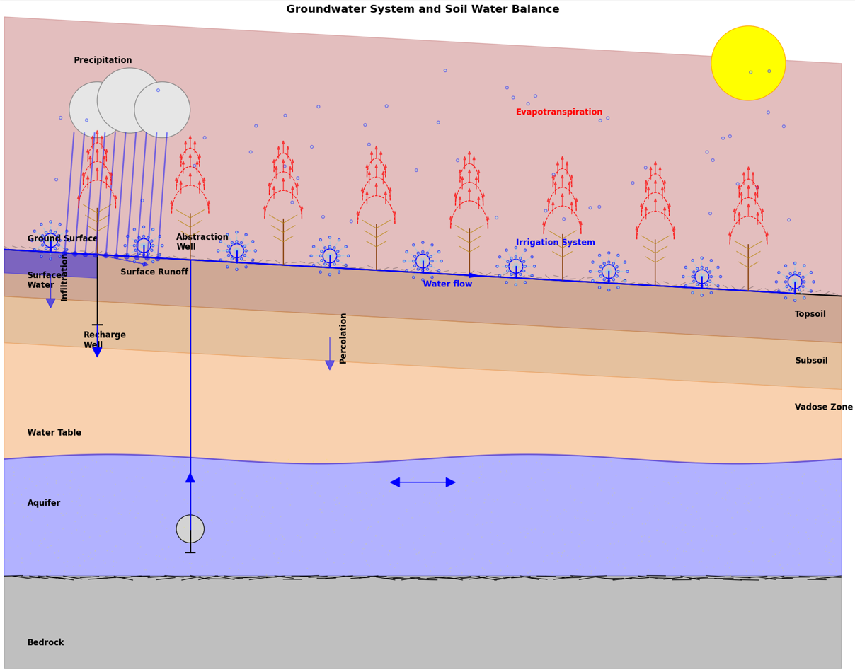
The figure provides a foundational visualization of the hydrological processes involved in understanding groundwater systems and soil water balance, which directly supports the methodologies discussed in Sections 4.2 and 4.3. Groundwater abstraction for irrigation use, as highlighted in Section 4.2, is depicted in the diagram through the abstraction well, showing the extraction of water from the aquifer. To accurately calculate groundwater abstraction for irrigation, the model incorporates crop water requirements, irrigation efficiency, and precipitation—processes represented visually by the precipitation and the irrigation system in the topsoil layer. Additionally, evapotranspiration is a critical parameter influencing water demand, shown in the diagram through upward red arrows representing water loss from soil and plants. This interplay informs the need for effective classification methods like AETI, which refine crop-specific water estimates.

Similarly, Section 4.3's focus on Groundwater Recharge aligns with the recharge well and the downward movement of water from infiltration and percolation depicted in the vadose zone of the diagram. The processes of precipitation, infiltration, and soil moisture dynamics, visualized in the figure, are key inputs for the Thornthwaite-Mather water balance model. The calculation of soil hydraulic properties (e.g., wilting point and field capacity) is essential for estimating recharge rates and is conceptually tied to the soil stratification (topsoil, subsoil, and vadose zone) and water movement into the aquifer. This integrated perspective of recharge and abstraction ensures the sustainable management of groundwater resources, as described in the methodologies.

4.2. Methodology of IGwA

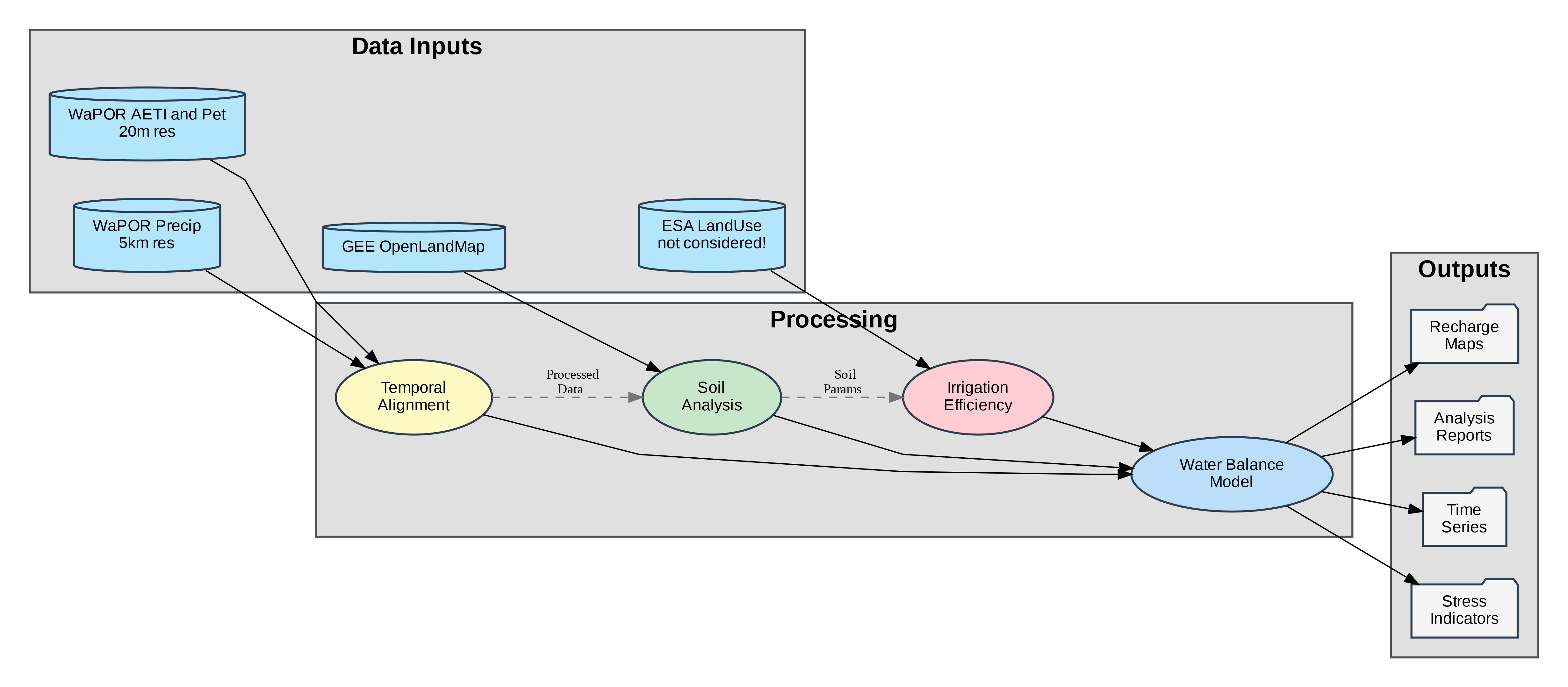
The following methodology provides a comprehensive framework for assessing groundwater dynamics in agricultural regions using remote sensing and hydrological modeling. The process begins with the integration of multi-source data, including high-resolution actual evapotranspiration (AETI) from WaPOR, daily precipitation from WaPOR, soil properties from GEE-OpenLandMap, and land-use classification from ESA (not included yet). These datasets are temporally aligned and spatially resampled to ensure consistency, forming the foundation for calculating critical parameters such as soil field capacity, wilting point, and irrigation efficiency. Key steps include the application of the Saxton & Rawls equations for soil hydraulic properties and crop-type-specific irrigation efficiency adjustments based on satellite-derived land-use data.

The core of the methodology employs an enhanced Thornthwaite-Mather water balance model to estimate groundwater recharge and abstraction. By analyzing the relationship between effective precipitation, potential evapotranspiration (PET), and soil moisture storage, the model iteratively calculates water deficits/surpluses while incorporating irrigation demands derived from AETI data. Irrigation efficiency is dynamically adjusted using crop-specific coefficients, improving the accuracy of abstraction estimates in arid agricultural systems. 

The final outputs—including spatially explicit recharge maps, abstraction rate time series, and water stress indices—provide actionable insights for sustainable groundwater management. This approach enables policymakers to identify over-exploited zones, optimize irrigation schedules, and assess climate change impacts on water resources. By leveraging Google Earth Engine’s cloud-computing capabilities, the methodology balances high spatial resolution (20m) with computational efficiency, making it particularly suitable for large-scale agricultural water management in data-scarce regions. The integration of calibration parameters and uncertainty analysis ensures robustness, while user-friendly visualizations facilitate stakeholder engagement and evidence-based decision-making.

---

4.3. Groundwater Abstraction for Irrigation

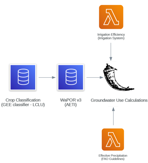
To estimate groundwater abstraction for irrigation purposes by analyzing crop water requirements, irrigation efficiency, and precipitation.

Methodology

The abstraction volume is calculated using crop water requirements, effective precipitation, and irrigation efficiency. Crop classification has to be the first step in determining water demand where a classification model is trained to identify crop types, with each type associated with specific water requirements. This process utilizes spectral-temporal statistics of satellite imagery. The classified crop map assigns water requirements.

In this model, the classification is considered by actual evapotranspiration (AETI) so the classifier procedures aren't implemented. While the model only incorporates AETI derived from WaPOR datasets, a significant area of improvement would be needed to involve dynamically linking AETI values to specific crop classifications. This could enhance the accuracy of water demand estimates and further refine the model.

 

4.4. Groundwater Recharge

To estimate groundwater recharge rates, incorporating precipitation, evapotranspiration, and soil moisture dynamics.

Methodology

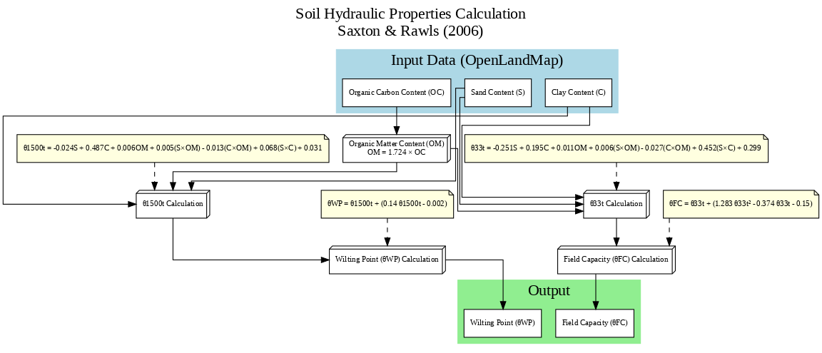
The following methodology integrates data from multiple sources and computational steps to estimate groundwater recharge using the Thornthwaite-Mather (TM) procedure. It begins with soil profile data obtained from OpenLandMap through Google Earth Engine (GEE) collections. This data undergoes preprocessing to adapt it for further analysis. Then, soil hydraulic properties such as wilting point and field capacity are calculated using the Saxton & Rawls (2006) approach. The results are utilized to determine the soil's hydraulic properties. Simultaneously, water availability data, including precipitation and potential evapotranspiration (PET), is derived from WaPOR v3. The computed soil and water data are combined in the TM procedure to model groundwater recharge.

 

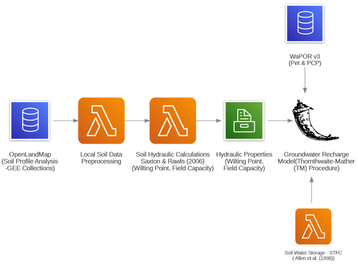
4.4.1 Hydraulic Properties (FC&WP) via Saxton-Rawls Model

 

OpenLandMap datasets are used to describe clay, sand and organic carbon content of soil. A global dataset of soil water content at the field capacity with a resolution of 250 m has been made available by Hengl & Gupta (2019). However, up to now, there is no dataset dedicated to the water content of soil at the wilting point. Consequently, in the following, both parameters will be determined considering the previous equations and using the global datasets giving the sand, clay and organic matter contents of the soil. According to the description, these datasets are based on machine learning predictions from global compilation of soil profiles and samples. Processing steps are described in detail here. The information (clay, sand content, etc.) is given at 6 standard depths (0, 10, 30, 60, 100 and 200 cm) at 250 m resolution.

Two key hydraulic properties of soil are utilized:

• the wilting point refers to the moisture level below which plants are unable to extract water through their roots.
• the field capacity marks the maximum moisture level that soil can retain. Beyond this point, gravitational forces prevail, causing water to percolate into deeper soil layers.

Equations developed by Saxton & Rawls (2006) are applied to correlate these parameters with soil texture. The wilting point water content, denoted as θWP, is calculated using the following formula:

with:

where:

• S: indicates the percentage of sand in the soil (by mass),
• C: represents the percentage of clay in the soil (by mass),
• OM: refers to the percentage of organic matter in the soil (by mass).

Likewise, the water content at field capacity, symbolized as θFC, is computed using this equation:

with:

Now that soil properties are described, the water content at the field capacity and at the wilting point can be calculated according to the equation defined at the beginning of this section. Please note that in the equation of Saxton & Rawls (2006), the wilting point and field capacity are calculated using the Organic Matter content (OM) and not the Organic Carbon content (OC). In the following, we convert OC into OM using the corrective factor known as the Van Bemmelen factor:

0M=1.724×OC

      

4.4.2 Soil Water Storage (STFC)

The soil water storage is calculated as outlined by Allen et al. (1998) (the document can be downloaded here):

TAW=1000×(θFC−θWP)×Zr

where:

• TAW: the total available soil water in the root zone [mm],

• θFC: the water content at the field capacity [m³m⁻³],

• θWP: the water content at wilting point [m³m⁻³],

• Zr: the rooting depth [m],

Typical values of θFC and θWP for different soil types are given in Table 19 of Allen et al. (1998).

The readily available water (RAW) is given by RAW=p×TAW, where p is the average fraction of TAW that can be depleted from the root zone before moisture stress (ranging between 0 to 1). This quantity is also noted as soil water storage (STFC) which is the available water stored at field capacity in the root zone.

Ranges of maximum effective rooting depth Zr, and soil water depletion fraction for no stress p, for common crops are given in the Table 22 of Allen et al. (1998). In addition, a global effective plant rooting depth dataset is provided by Yang et al. (2016) with a resolution of 0.5° by 0.5° (see the paper here and the dataset here).

According to this global dataset, the effective rooting depth around our region of interest can reasonably assumed to Zr=0.5. Additionally, the parameter p is also assumed constant and equal to and p=0.5 which is in line with common values described in Table 22 of Allen et al. (1998).

 

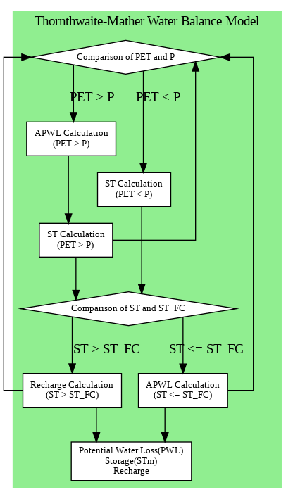
4.4.3 Thornthwaite-Mather (TM) Water Balance Model

The Thornthwaite-Mather procedure used to estimate groundwater recharge is explicitly described by Steenhuis and Van der Molen (1985). This procedure uses monthly sums of potential evaporation, cumulative precipitation, and the moisture status of the soil which is calculated iteratively. The moisture status of the soils depends on the accumulated potential water loss (PWL). This parameter is calculated depending on whether the potential evaporation is greater than or less than the cumulative precipitation. The procedure reads as follow:

The workflow follows these steps:

     1. Comparison of PET and P:

• The first step compares Potential Evapotranspiration (PET) and Precipitation (P) to determine whether the demand for water (PET) exceeds the supply (P) or not:

  • Case 1: PET > P

    • Water demand exceeds rainfall, triggering a calculation of APWL (Accumulated Potential Water Loss). This value tracks the cumulative water deficit due to evapotranspiration exceeding precipitation.
    • Soil water storage (ST) is updated based on the deficit.

  • Case 2: PET < P

    • Water supply exceeds demand, allowing for soil water storage (ST) replenishment.

      2. Comparison of Soil Water Storage (ST) with Field Capacity (ST_FC):

• After calculating or updating ST, it is compared with the Field Capacity (ST_FC):
  • Case 1: ST > ST_FC
    • When soil water storage exceeds field capacity, excess water is considered as Recharge, contributing to groundwater.
  • Case 2: ST ≤ ST_FC
    • When soil water storage is below or equal to field capacity, APWL is updated.

      3. Outputs:

• Based on the above conditions, the model computes:
  • Potential Water Loss (PWL): The water lost due to evapotranspiration when PET > P.
  • Soil Storage (STm): The updated soil water storage level.
  • Recharge: The water that contributes to replenishing groundwater when ST > ST_FC.

 

Use the following script to run the groundwater modeling using WaPOR and GEE

                                                      Python Script: Modeling Groundwater Abstraction for Irrigation and Recharge Using WaPOR and GEE

 

 

---